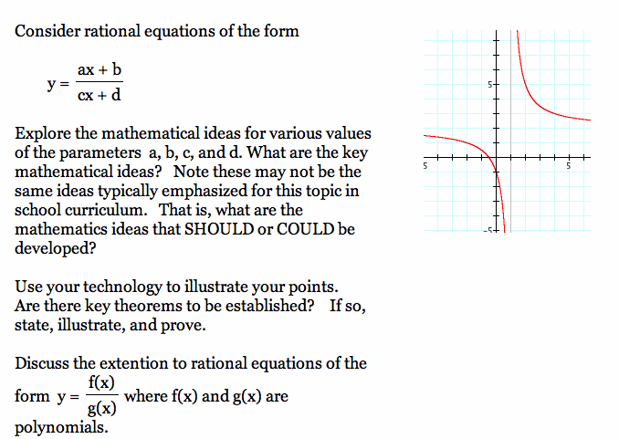
Final Assignment
Part 1


Final Assignment
Part 1

We will start our investigation by looking how the value of a affects the function. We will set a equal to -3, -2, -1, 2, 3, and 4. The values of b, c, and d will all be 1.


Click here for a movie that shows the value of a varying from -5 to 5. The graphs in the video have the same labels as the above graph.
Observations:
1. All of the functions have a vertical and horizontal asymptote. Recall that an asymptote is a line that the function approaches but never actually reaches.
2.The vertical asymptote for all of these functions is at x = -1. This is because all of the functions have the same denominator so the all of the functions are undefined at this value. If we set x equal to -1, we get 0 in the denominator and the function will be undefined.
3. The horizontal asymptote is different for each function. The asymptote appears to be at the line y = a. We will investigate this more later in the assignment to see if the value of a is always the horizontal asymptote.
4. The functions exists at all the x-values except at x = -1 so the domain of these functions is ![]() . The range for the functions will depend on the the horizontal asymptote. The horizontal asymptote for these functions is y = a so the range is
. The range for the functions will depend on the the horizontal asymptote. The horizontal asymptote for these functions is y = a so the range is ![]() .
.
5. The functions have the same y-intercept of 1. The x-intercept is different for each graph. The x-intercept can be found by setting the function equal to 0 and solving for x.
Now we will look at how the value of c changes the functions.
We will set a = b = d = 1 and c will be -3, -2, -1, 2, 3, and 4.


Click here for a movie that shows the value of c varying from -5 to 5. The graphs in the video have the same labels as the above graph.
Observations:
1. We notice that all of these functions have different vertical and horizontal asymptotes.
2. As we did in the first part, we can find the vertical asymptote by setting the denominator equal to zero and solving for x.
3. In the first part of the assignment, we noticed that the horizontal asymptote was at y = a. In these functions the horizontal asymptote is no longer the value of a. Instead the asymptote is y = a/c.
4. Unlike in the first part, the x-intercept and y-intercept are the same in all the functions.
Now lets look at how b affects the function.
We will set a = c = d = 1 and b will be -3, -2, -1, 2, 3, and 4.


Click here for a movie that shows the value of b varying from -5 to 5. The graphs in the video have the same labels as the above graph.
Observations:
1. These functions have the same vertical asymptote because the denominator is the same for each function.
2. The horizontal asymptote is also the same for all the functions because a = c = 1 so the horizontal asymptote is 1.
3. The only difference between these functions is the intercepts. The x-intercept can be found two ways. As we mentioned before, we can set y = 0 and solve for x. We can also just set the numerator equal to 0 and solve for x. Using this second way, it is easy to see that the x-intercept would change and would depend on the value of b. For example, if we set the numerator of the first function equal to 0 we have 0 = x - 3 so x = 3.
4. The y-intercepts is also different for the functions. We set x = 0 to find the y-intercept so it is easy to see that the y-intercept will be the value of b.
(Keep in mind that these observations are for when a, c, and d are 1)
Now lets look at how d affects the function.
We will set a = b = c = 1 and d will be -3, -2, -1, 2, 3, and 4.


Click here for a movie that shows the value of d varying from -5 to 5. The graphs in the video have the same labels as the above graph.
Observations:
1. The horizontal asymptotes are the same because a and c are both equal to 1 again.
2. The vertical asymptotes are different because we have changed the value of d. To find the vertical asymptote we set the denominator equal to 0 and solve for x. Since c = 1, the vertical asymptote will be the line x = -d.
3. The x-intercept for these functions is the same and is at -1. This is because a and b are both 1.
4. The y-intercepts are also different because the ratio of b/d is different for each function.
Conclusions:
1. To find vertical asymptote is found by setting the denominator equal to 0 and solving for x. So we'd get the line x = -d/c.
2. To find the horizontal asymptote look at the leading coefficient of the numerator and denominator. So we'd get the line y = a/c.
3. To get the x-intercepts set the the numerator equal to 0 and solve for x. So we'd get the point (-b/a, 0).
4. To get the y-intercepts set x = 0 and simplify. So we'd get the point (0,b/d).
Generalizations:
What if the expressions in the numerator and the denominator are not linear expressions? What if they are polynomials?
1. The vertical asymptotes can be found the same way by setting the denominator equal to zero and solving for x. However, since the degree is greater than 1, we could have more than 1 value for x so we would have more than 1 vertical asymptote. Here is an example of when this could happen:


As we can see, we have two vertical asymptotes at x = 4 and x = -4.
2. The x-intercepts and the y-intercepts can be found in the same way as if the expressions were linear. Again, we would have to be aware that we could have more than one x-intercept. Here is an example of when that would happen:


We can see the graph crosses the x-axis at -1 and 1. Because we are dealing with rational functions, we can never have more than one y-intercept. If we did have more than one than we would not be dealing with a function anymore.
3. Finding the horizontal asymptotes when the numerator and denominator are not linear is much different because we have to consider the degree of the polynomial in the numerator and denominator. There are three cases to consider: degree of the numerator and denominator are equal, the degree of the numerator is greater than that of the denominator, and the degree of the numerator is less than the degree of the denominator.
If the degrees are the same then we can proceed just as we did when we had linear expressions in the numerator and denominator (this makes sense because in those cases the degree was both 1). So the horizontal asymptote is equation y = a/c. Here is an example of this case:


As we can see, the function has a horizontal asymptote at y = 2.
If the degree of the polynomial in the numerator is greater than the degree of the polynomial in the denominator then we actually don't have any horizontal asymptotes. We have as slant asymptote. Here are some examples of when this happens:


If we have the degree of the polynomial in the numerator is less than the degree of the polynomial in the denominator than the horizontal asymptote is at y = 0. Here are examples of this:


As we can see, the horizontal asymptote is at y = 0.